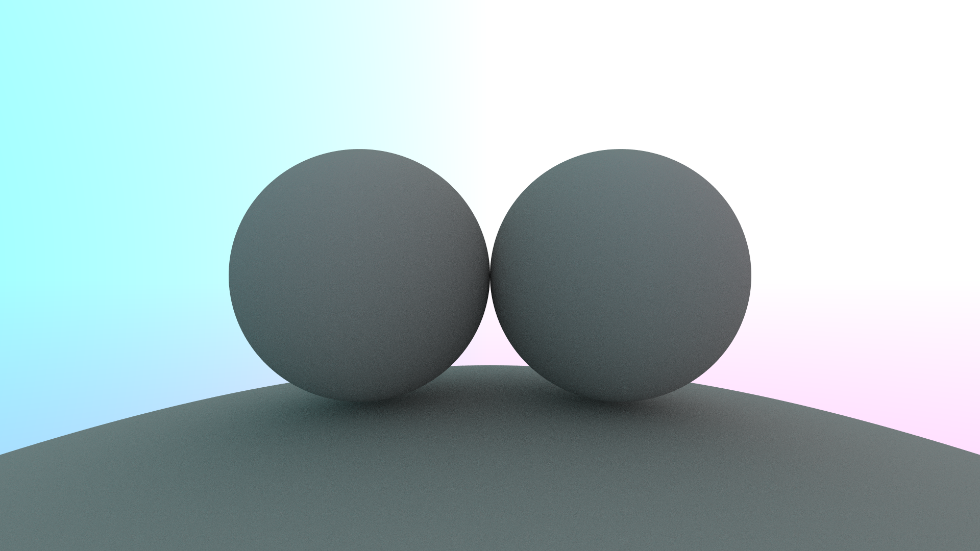
In last part we did the diffusion of ray from the surface, but it’s far from realistic. In this part, we will add some more realistic features to the ray tracing.
The Lambertian reflection is a model for diffuse reflection. It is more accurate than the previous model. The previous model was just scattering the ray in random direction, but the Lambertian reflection model scatters the ray in a direction that is proportional to the cosine of the angle between the incoming ray and the normal of the surface, which is reasonable because the reflection is more likely to be in the direction of the normal.
In this graphic, we have CP the incident ray, PN, the normalized normal of the surface, and the pink lines showing the magnitude of probability of choosing this direction to reflect. We can see when the angle between the incident ray and the normal is small, the reflection is more likely to be in the direction of the normal.
The implementation is very simple. We pick the normalized normal vector of the surface and add a random unit vector to it (blue vectors in the graphic). And here is the code:
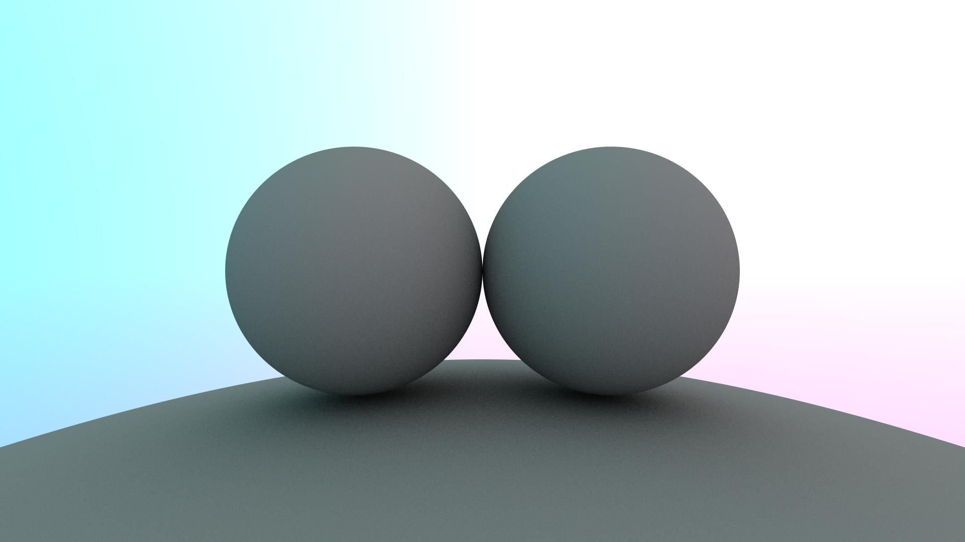
If we use a color picker to check the surface color of the two sphere, we will see that the color is not exactly what we expected. My check yields 100, 107, 110, which is approximately half way, but this should be more half way because the intensity decrease by one half each time it reflects, yet we have a bright environment.
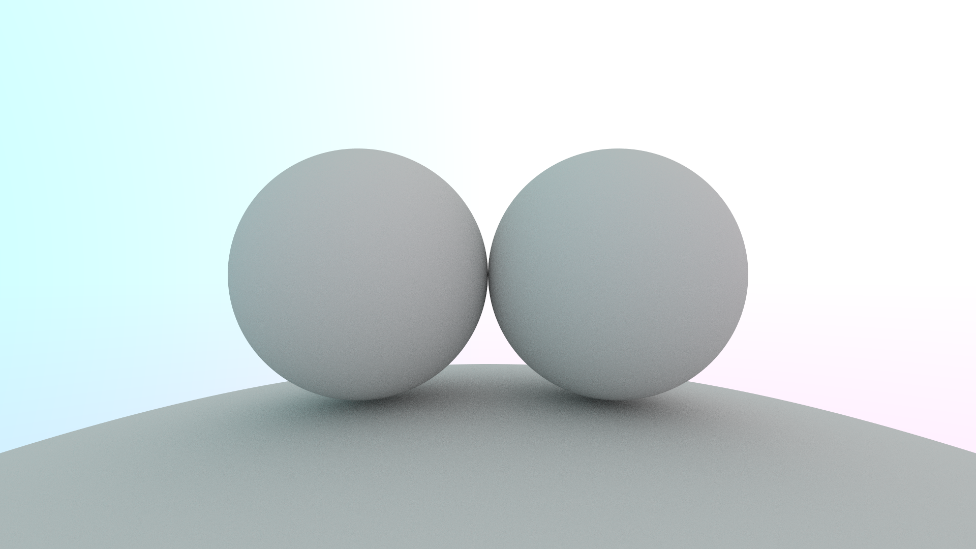
This will occur because there is a space called gamma space, which the image viewer assume the image is in. However, recall our image generator, which the color intensity increases linearly as each color increases linearly. This is called linear space. The difference between these two space is the gamma correction, a mapping from linear space to gamma space. In this case we will use gamma = 1/2.2.
The code is simple, we just need to apply the gamma correction to the color before we write it to the image file:
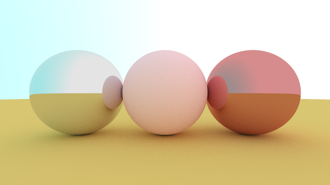
Material is how the surface of the object interacts with the light. For example, our current model is a diffuse material, which uses Lambertian reflection. There are other materials, such as metal, glass, and so on. We will implement a metal material in this part.
First, we will implement an interface for materials, a material will determine how much the ray is reflected, and how the ray is reflected. We will use the interface to implement the material:
In this case, our Lambertian material will do the same thing. A material can either choose to absorb the ray, or to diffuse the ray, or do both. In our case, we will only diffuse the ray.
Notice that we calculated ray direction, by adding a random unit vector to the normal of the surface. However, if we are extremely unlucky, the ray direction will be in the opposite direction of the normal. In this case, the result is not good. We can fix this by checking whether the magnitude of the ray direction is very small, and if it is, we will just use the normal of the surface as the ray direction. This will make the result more realistic.
The next material we will implement is the metal material. In this case, the metal material will reflect the ray in a direction. We know there is a law called the law of reflection, which states that the angle of incidence is equal to the angle of reflection, illustrated in this graphic:
With this graph it’s not hard to see that the reflected ray direction vector is:
R=I−2⋅H
we know H is normal to the surface, and it has same y conponent as I, so we can write H as:
Some metal doesn’t do full reflect, especially unpolished metal. Adding a fuzziness factor to the metal material will make the reflection less sharp. Since for metal, we need to reach fuzziness and reflection at the same time, we can do the following:
Do the reflection as normal
Add a random unit vector to the reflected ray direction, and multiply it by the fuzziness factor to manipulate the diversion of the reflected ray
icon-padding
In this case, the dashed pink vector is the original reflected ray direction, and vector RD is the fuzziness vector(with the randomness factor to be 1). The final reflected ray direction is the sum of the two vectors, or the blue vector.
We will add a fuzziness member variable to the Metal material, and modify the scatter function to use it: